Themes in R Histogram With Continuous Fill

GGPlot Histogram

A histogram plot is an alternative to Density plot for visualizing the distribution of a continuous variable. This chart represents the distribution of a continuous variable by dividing into bins and counting the number of observations in each bin.

This article describes how to create Histogram plots using the ggplot2 R package.

Contents:

• Key R functions
• Data preparation
• Loading required R package
• Basic histogram plots
• Change color by groups
• Combine histogram and density plots
• Conclusion

Related Book

GGPlot2 Essentials for Great Data Visualization in R

Key R functions

• Key function: geom_histgram() (for density plots).
• Key arguments to customize the plots:
  • color, size, linetype: change the line color, size and type, respectively
  • fill: change the areas fill color (for bar plots, histograms and density plots)
  • alpha: create a semi-transparent color.

Data preparation

Create some data (wdata) containing the weights by sex (M for male; F for female):

                  set.seed(1234) wdata = data.frame(         sex = factor(rep(c("F", "M"), each=200)),         weight = c(rnorm(200, 55), rnorm(200, 58))         )  head(wdata, 4)                

                  ##   sex weight ## 1   F   53.8 ## 2   F   55.3 ## 3   F   56.1 ## 4   F   52.7                

Compute the mean weight by sex using the dplyr package. First, the data is grouped by sex and then summarized by computing the mean weight by groups. The operator %>% is used to combine multiple operations:

                  library("dplyr") mu <- wdata %>%    group_by(sex) %>%   summarise(grp.mean = mean(weight)) mu                

                  ## # A tibble: 2 x 2 ##   sex   grp.mean ##   <fct>    <dbl> ## 1 F         54.9 ## 2 M         58.1                

Loading required R package

Load the ggplot2 package and set the default theme to theme_classic() with the legend at the top of the plot:

                  library(ggplot2) theme_set(   theme_classic() +     theme(legend.position = "top")   )                

Basic histogram plots

We start by creating a plot, named a, that we'll finish in the next section by adding a layer using the function geom_histogram().

                  a <- ggplot(wdata, aes(x = weight))                

The following R code creates some basic density plots with a vertical line corresponding to the mean value of the weight variable (geom_vline()):

                  # Basic density plots a + geom_histogram(bins = 30, color = "black", fill = "gray") +   geom_vline(aes(xintercept = mean(weight)),               linetype = "dashed", size = 0.6)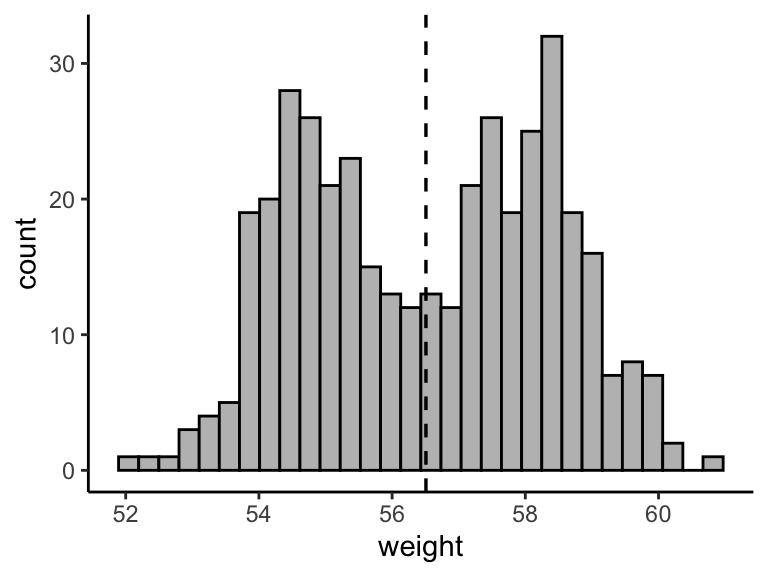                

Note that, by default:

• By default, geom_histogram() uses 30 bins - this might not be good default. You can change the number of bins (e.g.: bins = 50) or the bin width (e.g.: binwidth = 0.5)
• The y axis corresponds to the count of weight values. If you want to change the plot in order to have the density on y axis, specify the argument y = ..density.. in aes().

Change color by groups

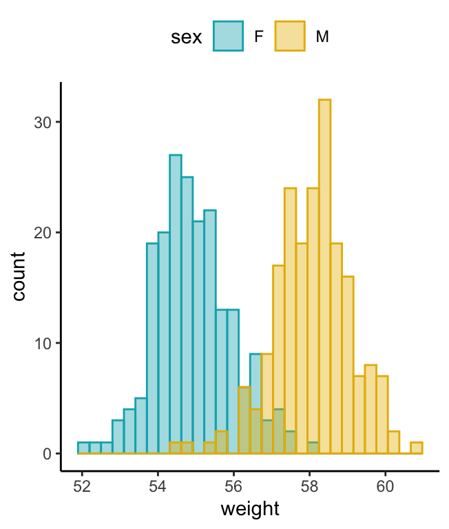
The following R code will change the histogram plot line and fill color by groups. The functions scale_color_manual() and scale_fill_manual() are used to specify custom colors for each group.

We'll proceed as follow:

• Change areas fill and add line color by groups (sex)
• Add vertical mean lines using geom_vline(). Data: mu, which contains the mean values of weights by sex (computed in the previous section).
• Change color manually:
  • use scale_color_manual() or scale_colour_manual() for changing line color
  • use scale_fill_manual() for changing area fill colors.
• Adjust the position of histogram bars by using the argument position. Allowed values: "identity", "stack", "dodge". Default value is "stack".

                  # Change line color by sex a + geom_histogram(aes(color = sex), fill = "white",                    position = "identity") +   scale_color_manual(values = c("#00AFBB", "#E7B800"))   # change fill and outline color manually  a + geom_histogram(aes(color = sex, fill = sex),                          alpha = 0.4, position = "identity") +   scale_fill_manual(values = c("#00AFBB", "#E7B800")) +   scale_color_manual(values = c("#00AFBB", "#E7B800"))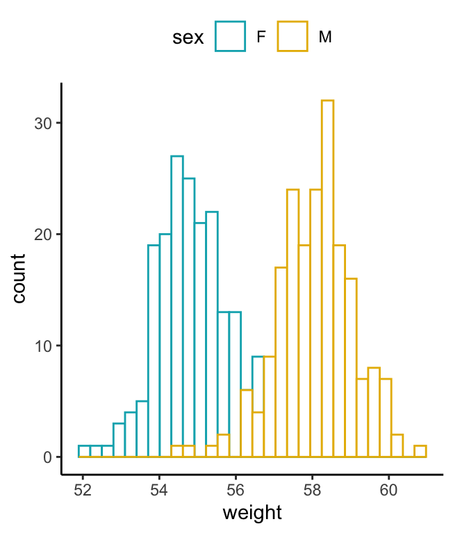                

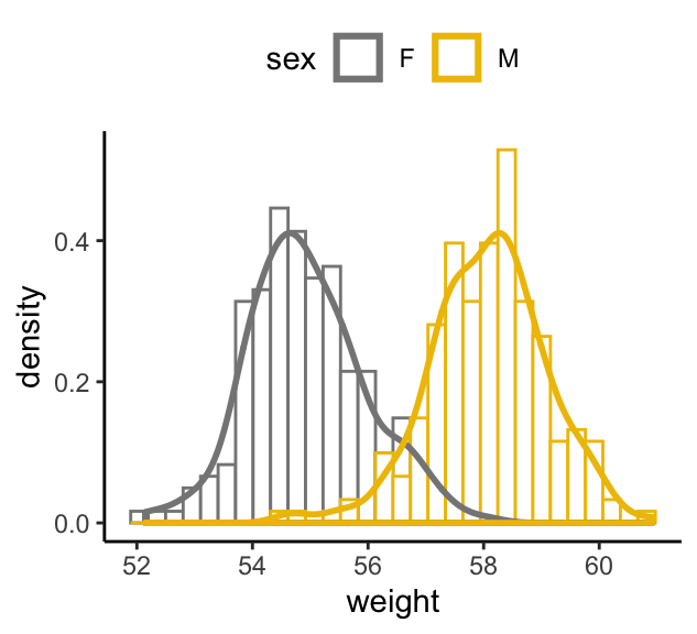
Combine histogram and density plots

• Plot histogram with density values on y-axis (instead of count values).
• Add density plot with transparent density plot

                  # Histogram with density plot a + geom_histogram(aes(y = stat(density)),                     colour="black", fill="white") +   geom_density(alpha = 0.2, fill = "#FF6666")         # Color by groups a + geom_histogram(aes(y = stat(density), color = sex),                     fill = "white",position = "identity")+   geom_density(aes(color = sex), size = 1) +   scale_color_manual(values = c("#868686FF", "#EFC000FF"))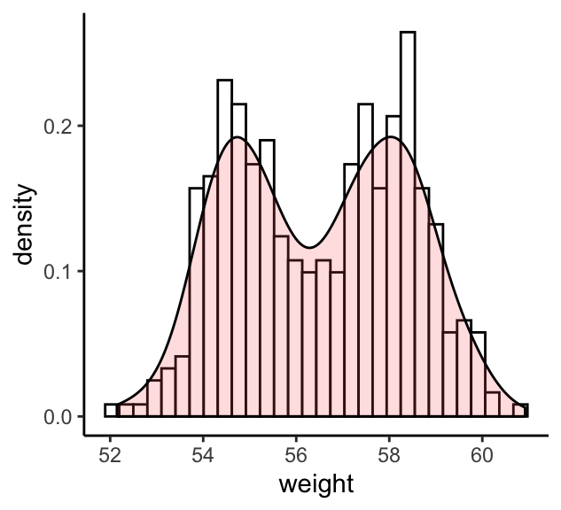                

Conclusion

This article describes how to create histogram plots using the ggplot2 package.

Recommended for you

This section contains best data science and self-development resources to help you on your path.

Version: Français

Back to Data Visualization using GGPlot2

mccloudmakenhaved1960.blogspot.com

Source: https://www.datanovia.com/en/lessons/ggplot-histogram/

Share this post